
ENVIRONMENT AND ENERGY
Direct Numerical Simulation of Coupled Land–Atmosphere Systems
Principal Investigator:
Cedrick Ansorge
Affiliation:
Institute of Geophysics and Meteorology, University of Cologne (Germany)
Local Project ID:
hku24
HPC Platform used:
JUWELS and JUQUEEN of JSC
Date published:
1. Surface-Atmosphere Interaction in The Earth System
The estimation of exchange between the land surface and the atmosphere is a crucial task in numerical modelling of atmospheric flow and eminently linked to the yet unsolved problem of turbulence closure in classical physics: Exchange at the surface determines the transport of heat, water vapor, momentum and pollutants to the atmosphere and thus the availability of these quantities in the boundary layer, the lowest part of the earth atmosphere. The distribution of heat, momentum, vapor and pollutants has immediate impact locally, but also on the large-scale weather through cloud and rain formation or the genesis or dissipation of weather systems. But, the distribution of these agents is also relevant for potentially hazardous events such as frost, fog or haze.
To represent the surface exchange, a theoretical framework based on strong assumptions about turbulence in vicinity of the surface is commonly used that was developed in the 1950s by Andrey Monin and Alexandr Obukhov (Monin—Obukhov Similarity Theory1, MOST). Motivated by point measurements on meteorological masts—still today the most common approach to determine the atmospheric state through in-situ observations—MOST is conceptually designed in an ensemble-averaged context, i.e. it is only valid over a large number of realizations of the same problem or, applying the ergodic hypothesis, for a large one- or two-dimensional average.
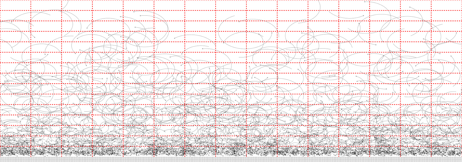
Figure 1. Schematic of turbulent eddies (swirly air motions) in the planetary boundary layer and a gridded representation of the flow as it is for instance achieved in Large-Eddy Simulation.
Figure reproduced from Ansorge (2019)7; license: CC BY 4.0
Non-local effects due to advection are neglected as well as the impact of local land-surface heterogeneity. This limit is, however, rarely encountered in the coupled land-atmosphere system which is characterized by heterogeneities on all scales ranging from the millimeter range to the global land/sea, orographic and vegetation patterns. Accounting for these heterogeneities and associated processes and interactions, both the atmospheric and surface components of coupled land–atmosphere systems have evolved at an increasing pace over the past few decades in terms of complexity and increasing resolution. But MOST is still the essential methodology communicating perturbations, and not only the mean state, in between the land and atmospheric components of such models. Despite these known conceptual and practical deficiencies, MOST is commonly used to estimate surface fluxes under real-world conditions in virtually all global circulation models and also large-eddy simulation (LES) of atmospheric boundary-layer flow. We inquire here: To what extent is the representation of surface—atmosphere exchange through MOST incorrect due to its application at small scales for which the theory is not applicable from a strict perspective?
2. The Role of Turbulence in Surface-Atmosphere Coupling
It turns out that it is actually turbulence which governs the exchange in vicinity of the surface; and turbulence occurs on a tremendously wide range of scales. At the range of weather patterns (100-1000km), turbulent motion earns its energy from instability processes that eventually cause the swirly character of turbulent flow as it is perceived in the form of swirling leaves during autumn or bumpy flight episodes due to a cascade of instabilities. These swirly motions break down and fill the range of scales towards smaller and smaller motion (as illustrated in Figure 1) until they start to feel the viscosity of air and their kinetic energy is dissipated to heat. This happens at the so-called Kolmogorov scale (named after Andrey N. Kolmogorov who came up with a mathematical description of this process in his famous 1941 paper 2)—typically on the order of a millimeter in atmospheric conditions.
To yield a tractable representation of the earth system in terms of a discrete grid (for instance given by the red dashed lines in Figure 1), the cascade of motions is truncated, i.e. only the largest scales—those that force the system energetically—are considered. Such truncated equations are, however, not closed in a mathematical sense; there appear to be more unknowns than equations as a consequence of the truncation. To close the equations, i.e. increase the number of equations such that the system becomes solvable, one can represent turbulent mixing by knowns variables. That means, one approximates the effect of turbulence using known variables and certain assumptions that depend on the resolution, but also mirror the particular purpose of a model. This procedure is called turbulence closure through mixing parameterization: the equations of motion are closed in a mathematical sense (number of unknowns is reduced to match the number of equations) by expressing the mixing terms through parameters of the modelled flow. The underlying assumptions most prominently include that the mixing which is represented through the parameterization be stationary (i.e. it does not change over time) and homogeneous (i.e. it does not change in space).
The challenge in modelling the surface—atmosphere interaction is that it eventually happens at the surface where there is no explicit representation of the mixing processes in numerical models of the earth system as they are used for weather prediction, climate projection or process studies in the field of geosciences. As seen schematically in Figure 1, the mixing elements in vicinity of the surface are very small, a requirement that is caused by the presence of the wall which suppresses any kind of motion: In immediate vicinity of a wall the velocity of the air has to match that of the wall which sets both velocities equal zero. This absence of large-scale mixing elements requires all turbulent exchange at the wall to be parameterized. Hence, MOST completely determines this crucial parameter of the atmospheric boundary layer, and is not only used for large-scale applications, but also to represent the surface-atmosphere interaction in smaller-scale applications such as LES models investigating the interaction between the surface and the atmosphere. When inquiring about the role or accuracy of MOST, these tools are not usable for they employ MOST. Hence, indirect approaches (for instance based on the identification of internal inconsistencies3) or other tools have to be used for such inquiry.
3. Numerical Simulation of Turbulence – a Problem of Scale
A novel avenue that became available with the advent of massively parallel supercomputing is the direct numerical simulation of a turbulent flow (cf. Figure 2), i.e. the problem is not solved on the red grid schematically shown in Figure 1, but on a grid that represents the entire range of motions, i.e. one that can resolve all eddies present in the turbulent boundary layer.
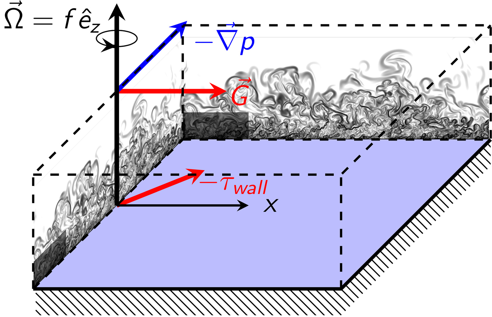
Figure 2. Schematic of the set-up used for direct numerical simulation. The flow is considered aloft a flat plate, rotating about its wall-normal axis ez at a rate f. The mean wind G is driven by a large-scale pressure gradient ∇p and, in absence of other forces, it is balanced by the Coriolis force. In vicinity of the wall, friction comes into play and the wind slows down such that the Coriolis force is reduced and the wind turns in favor of the pressure gradient.
Figure reproduced from Ansorge (2019)7; license: CC BY 4.0
Still today, such approach is not feasible in an exact sense, but only approximately: An order of magnitude estimation of the degrees of freedom in an atmospheric boundary-layer flow based on the largest and smallest scales (103 m / 10-3 m = 106 ) yields about 1018 degrees of freedom in space on a discrete cartesian grid. Representing and integrating such large problems over time is—and it will remain so for the foreseeable future, no matter what growth of resources one expects—not possible on a modern supercomputer. But the immense range of scales present in geophysical systems allows another approach to be taken, namely Reynolds-Number similarity: a similar problem is solved cutting the spectrum of motion at larger scale. Physically, this can be seen as using a more viscous fluid, for instance honey instead of air. If this problem has a sufficiently large number of degrees of freedom (that can be estimated from rigorous mathematical instability theory4-6), then some integral quantities such as velocity profiles and the exchange of turbulent motion on larger scales may be represented satisfactorily.

Figure 3 Two-dimensional field of total horizontal wind speed H ≡ (u2+v2)1/2 (left panels, a and c, shown in range 0.5 < H < 1 from blue to yellow) and wall friction velocity u*/G (right panels, b and d, shown in the range (0.03 < u*/G < 0.07 from blue to yellow). Upper panel shows 1 x 1/2 of the full simulation domain; Lower panel shows 1/8 x 1/16 of the domain as indicated by the dashed lines in the lower panel. The full domain consists of 2560 x 5120 grid points.
Figure reproduced from Ansorge (2019)7; license: CC BY 4.0
Recent work on atmospheric flow shows that direct numerical simulation with a scale separation of about 103 (yielding about 109 degrees of freedom in three-dimensional space) indeed exhibits such scale similarity. This allows to reduce geophysical turbulence problems to a size tractable on the super-computers of the Jülich Supercomputing Centre (JSC). We use this approach as a virtual lab to assess aspects of the geophysical problem that are hardly observable in the field due to either measurement issues or process interactions that hamper the attribution of observed effects to a particular physical phenomenon.
4. A Question of Scale? Insights on Scale-Dependency of Surface—Atmosphere Coupling from DNS
The direct representation of turbulent motion on all scales allows us to quantitatively assess the turbulent flow and to analyze a priori the validity and precision of MOST. The key approach in MOST is to close for the turbulent flux by linking it to the mean wind at a height in the logarithmic region (the straight section of the green line in Figure 4). With all data, i.e. both the wall stress and the velocity field, at hands, we can directly assess this assumption: In Figure 3, the wind pattern in the lower turbulent boundary layer (left) is shown together with the surface momentum flux, i.e. the surface—atmosphere exchange of momentum. While there certainly is a resemblance of the pattern at large scale (upper row), the features at small scale look much different. The narrow streaks in surface stress (lower right) correspond to a swirly pattern in the wind field. Talking in terms of the vertical wind profiles, the postulated linkage of surface stress and wind in the boundary layer would imply that a lower velocity within the boundary layer (say at y+ = 50) should correspond to a lower stress at the surface and thus less wind in immediate vicinity of the surface.
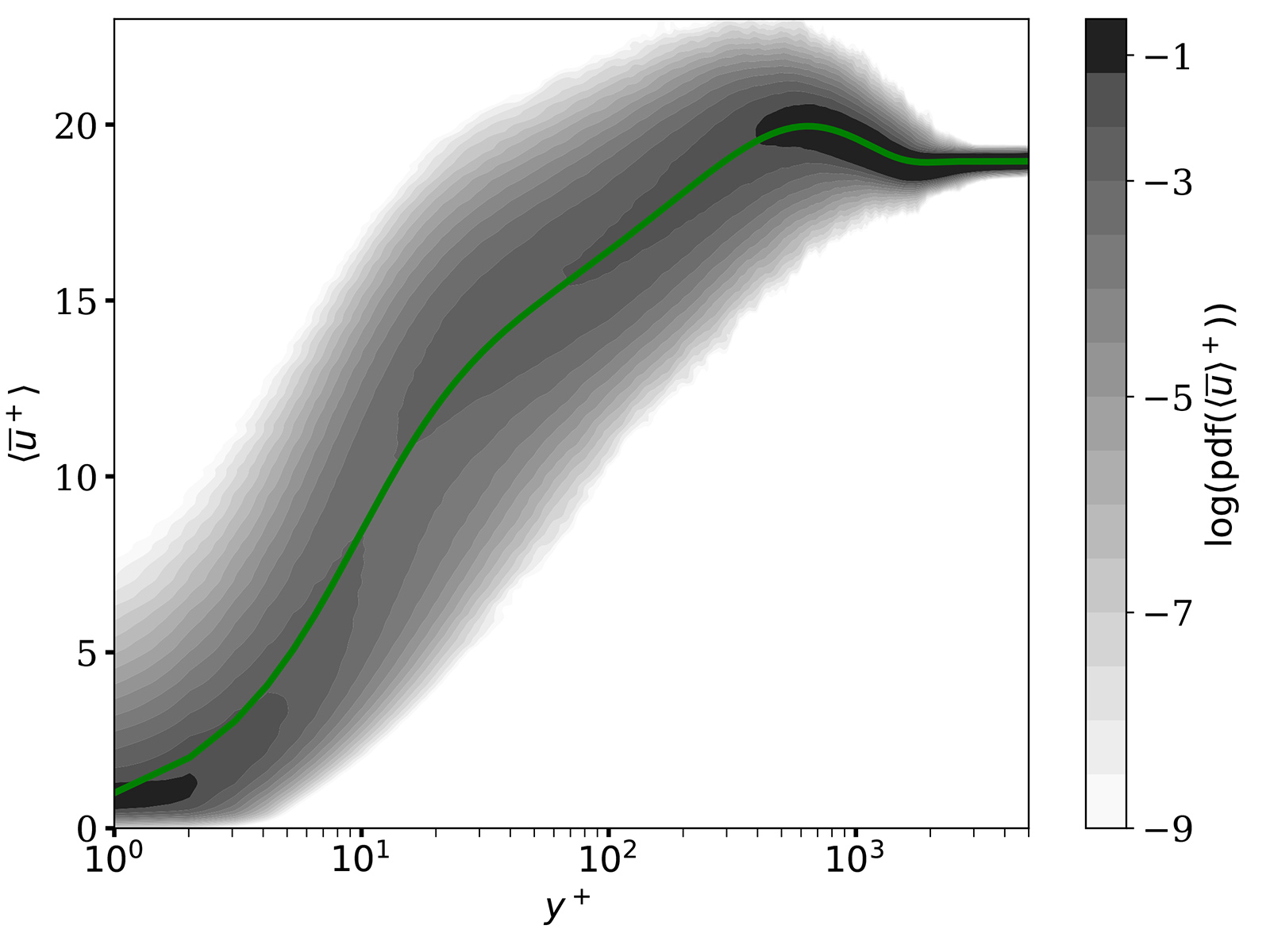
Figure 4. Probability of wind velocity at a certain height (white stands for no probability, light gray regions are rare and black regions very common). The mean wind profile is shown as a green line.
Figure reproduced from Ansorge (2019)7; license: CC BY 4.0
Through our compute project at FZJ, a plethora of data has been generated through direct numerical simulation of the flow in a broad range of conditions representative of the various dynamical states the atmospheric boundary layer can take. Based on this data, this key feature of surface-atmosphere coupling was quantitatively analyzed in our project7. We unveil that for neutral and near-neutral conditions—when there is no strong temperature inversion, but also no strong heating from the surface—, the averaging hypotheses underlying MOST are valid and correct estimates of coupling for the mean state of surface flux and boundary-layer winds are possible. The critical scale beyond which this averaging has a sufficient sample is found to be on the order of 10m. For most applications in atmospheric science, such as large-scale models or large eddy simulation (LES), this is sufficient. Care must, however, be taken for very-high-resolution approaches where the turbulence is parameterized, a more and more common approach in process studies of boundary-layer processes.
While large-scale models such as numerical weather prediction and climate projection are concerned with a prediction or projection of the mean state, LES approaches also are concerned with the local variability. Our comprehensive data analysis but shows that the resolved variance of these quantities is not propagated accurately. The error in variance is approximately proportional to the logarithm of height which follows from Townsend’s attached-eddy hypothesis (indeed, our work can thus also be seen as another confirmation of Townsend’s hypothesis, a corner stone of quantitative boundary-layer theory).
When stable stratification enters the problem—this is the case when the surface cools down rapidly as happens around sunset on clear days or due to advection of warm air over a cold surface—, large-scale structures form in the boundary-layer wind fields, and the organization of these structures appears to be governed from aloft rather than from the surface. In consequence, there is no means to predict these large-scale features in the boundary layer from the surface signal, and the approach fails to predict any local variation, while the mean state is constrained relatively well.
5. A Question of Direction? The Boundary layer appears different whether we look at it through point, Ensemble or Plane averages
We have seen that it is essential to consider a sufficiently large sample for atmosphere-surface coupling through MOST, which means, it should never be applied to scales less than the order of 10m; and for stable conditions, in fact, only to an average over a scale that is representative of the bulk boundary-layer state. The question arises then, How to average? Atmospheric observations are most accurately and commonly obtained through point measurements with a coarse vertical resolution and limited extent set by the height of measurement towers. In numerical simulation, horizontal averages over planes are common, but in principle any kind of sampling is possible. In our project, we exploit this capability of numerical simulation to analyze whether the direction of averaging has an impact on the surface-atmosphere coupling and its representation through MOST which is theoretically based on the ensemble average. When this two-dimensional average is considered, indeed the correlation between the surface-stress and the wind in the boundary layer approximately approaches 1.0 at very large scale (a filtering scale on the order of 103-104; cf. Figure 4). This is definitely not the case when only considering the correlation along lines and a crucial problem of averaged boundary-layer-structure properties: the structures forming turbulence, even in immediate vicinity to the wall, have a systematic tilt. Such miscorrelation is problematic when using vertical profiles which cannot be compensated for by an extension of the averaging period. If, however, the second dimension is taken into account, the effect of this tilt is covered by the averaging procedure. This limitation is crucial for the interpretation of turbulence measurements from towers.
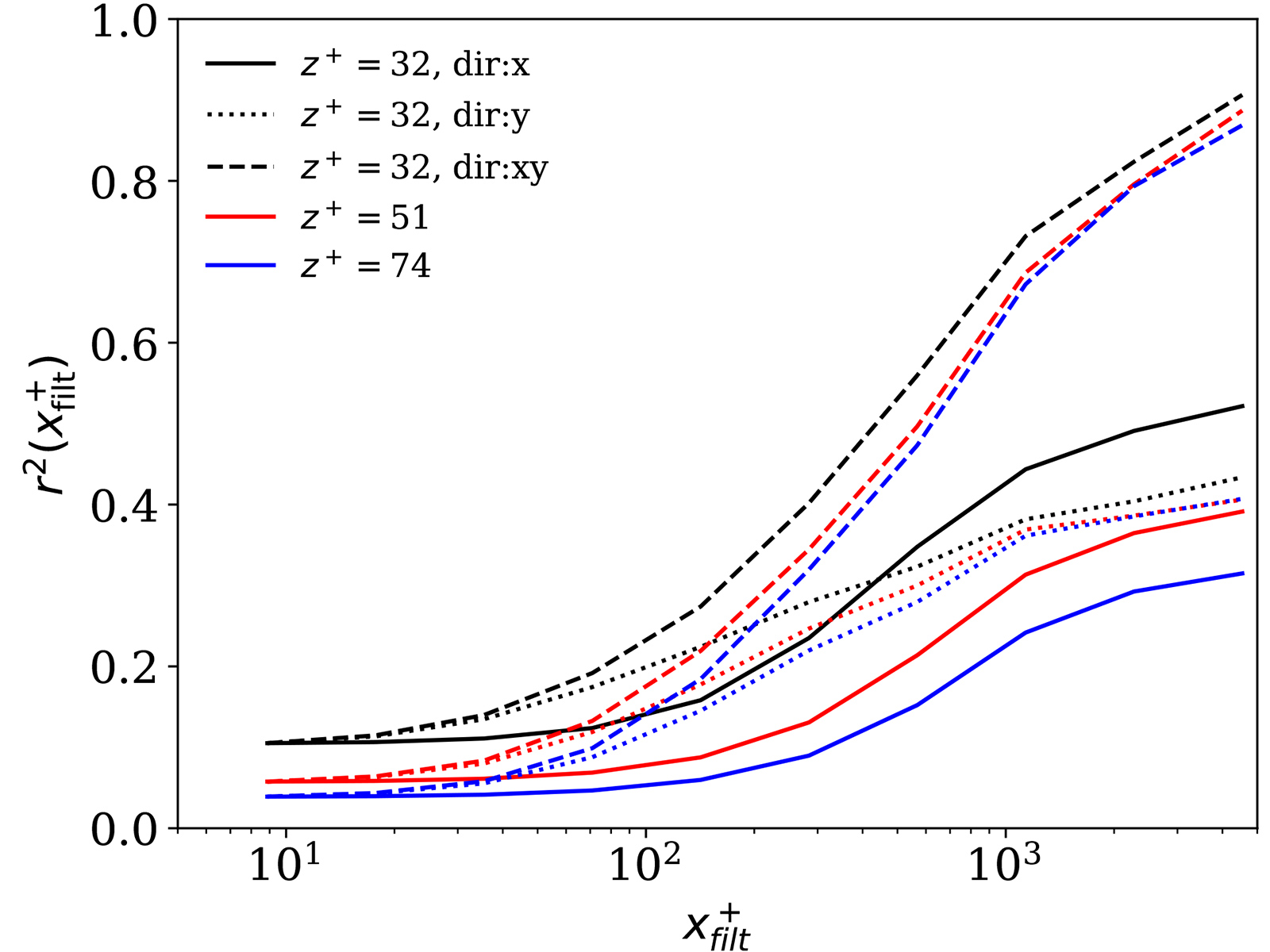
Figure 5. Correlation of the surface shear stress with the boundary-layer wind as a function of averaging scale. The dashed line is for a two-dimensional (horizontal-plane) average whereas the solid lines show the averages along the direction of the mean wall stress and perpendicular to it.
Figure reproduced from Ansorge (2019)7; license: CC BY 4.0
6. Synthesis
We have exemplified here the outcomes achieved when turbulence-resolving simulation of a three-dimensional flow is used to inquire about particular properties of the atmospheric boundary layer. The focus is on surface—atmosphere interaction, a key issue in numerical modelling of atmospheric flow—be it for numerical weather prediction, climate projection or for process-level inquiry by Large-Eddy Simulation. Not only provides our work valuable practical limits of applicability for Monin—Obukhov similarity theory but also it quantifies the error due to violation of these limits. While this is of immense practical use for applications of surface-layer theory, the utility of data generated as part of our project is not limited to this particular question. Turbulent Ekman flow is understudied in comparison to other canonical turbulent flows such as plane Couette flow, pipe flow or channel flow, but it is the flow that most closely resembles the atmospheric boundary-layer. The stably stratified atmospheric boundary layer is a phenomenologically rich and intricating system characterized by scale-interactions and process coupling such as wave-turbulence interaction or local laminarization. Such phenomena yet pose a great challenge to modelling surface atmosphere exchange, and it occurs that for a process-level study of these a correct representation of the small-scale turbulence is inevitable. We will hence continue to use the data in pursuit of these pressing questions in boundary-layer meteorology.
References
1. Monin, A. S. & Obukhov, A. M. Osnovnye zakonomernosti turbulentnogo peremeshivanija v prizemnom sloe atmosfery (Basic Laws of Turbulent Mixing in the Atmosphere Near the Ground). Trudy geofiz. inst. AN SSSR 24, 163–187 (1954).
2. Kolmogorov, A. N. Dissipation of Energy in locally isotropic turbulence. Dokl Akad Nauk SSSR 32, 19–21 (1941).
3. Shao, Y., Liu, S., Schween, J. H. & Crewell, S. Large-Eddy Atmosphere–Land-Surface Modelling over Heterogeneous Surfaces: Model Development and Comparison with Measurements. Boundary-Layer Meteorol 148, 333–356 (2013).
4. Di Prima, R. C. & Swinney, H. L. in Hydrodynamic Instabilities and the Transition to Turbulence (eds. Swinney, H. L. & Gollub, J. P.) (Springer-Verlag, 1981).
5. Lilly, D. K. On the Instability of Ekman Boundary Layer Flow. J Atmos Sci 23, 481–494 (1966).
6. Taylor, G. I. Stability of a viscous liquid contained between two rotating cylinders. Philosophical Transactions of the Royal Society of London A: Mathematical, Physical and Engineering Sciences 223, 289–343 (1923).
7. Ansorge, C. Scale Dependence of Atmosphere–Surface Coupling Through Similarity Theory. Boundary-Layer Meteorol 170, 1–27 (2019).
Scientific Contact:
Dr. Cedrick Ansorge
Institute of Geophysics and Meteorology
University of Cologne
Pohligstr. 3, D-50969 Köln (Germany)
e-mail: cansorge [@] uni-koeln.de
JSC Project ID: hku24
July 2019